On this page, I will briefly show how to populate the dimensions with data, and how to populate the cube.
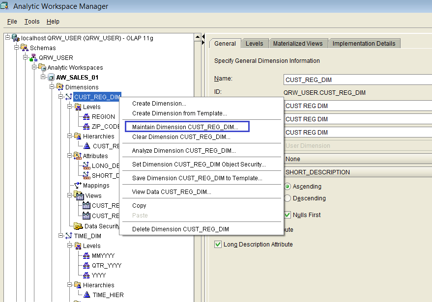
Figure 21 below shows the pop-up menu we get when we select dimension CUST_REG_DIM and then we click the right button on the mouse.
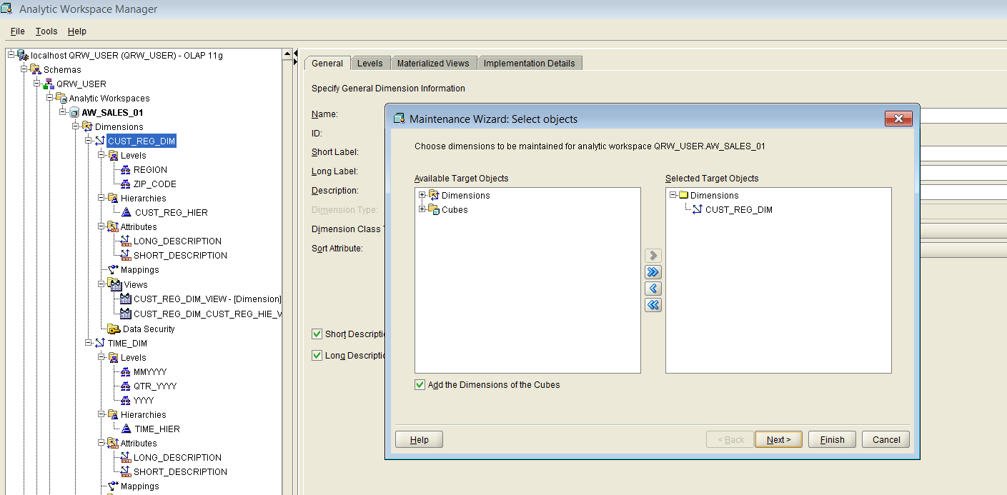
If we choose the item “Maintain Dimension CUST_REG_DIM” from the pop-up menu, then a wizard-style window appears, as shown below in Figure 22.
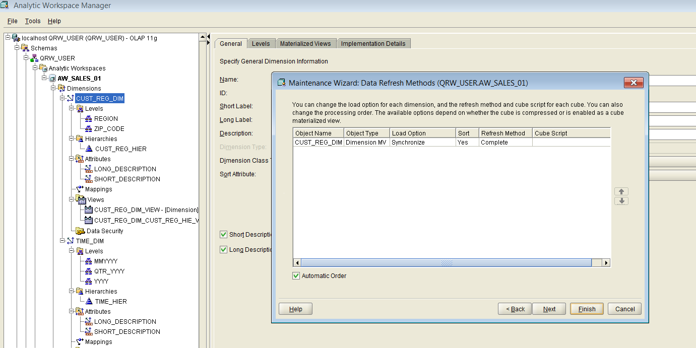
We choose dimension CUST_REG_DIM from the available objects, we add it to the right pane, and then we click “Next”, which brings us to the second step of the wizard, as shown below in Figure 23:
We can now click on the “Finish” button, which will initiate the loading of dimension CUST_REG_DIM with data.
We repeat the steps described above, for dimension TIME_DIM.
By now, we should have loaded both dimensions CUST_REG_DIM and TIME_DIM with data.
Please note that, in order for the loading of the dimensions with data to succeed, the column mappings of both dimensions to source tables must have been done according to the screen captures from the previous pages. The same goes for the mappings of the cube to the source tables.
The next steps are to build the cube CB_SALES_2, and to load it with data.
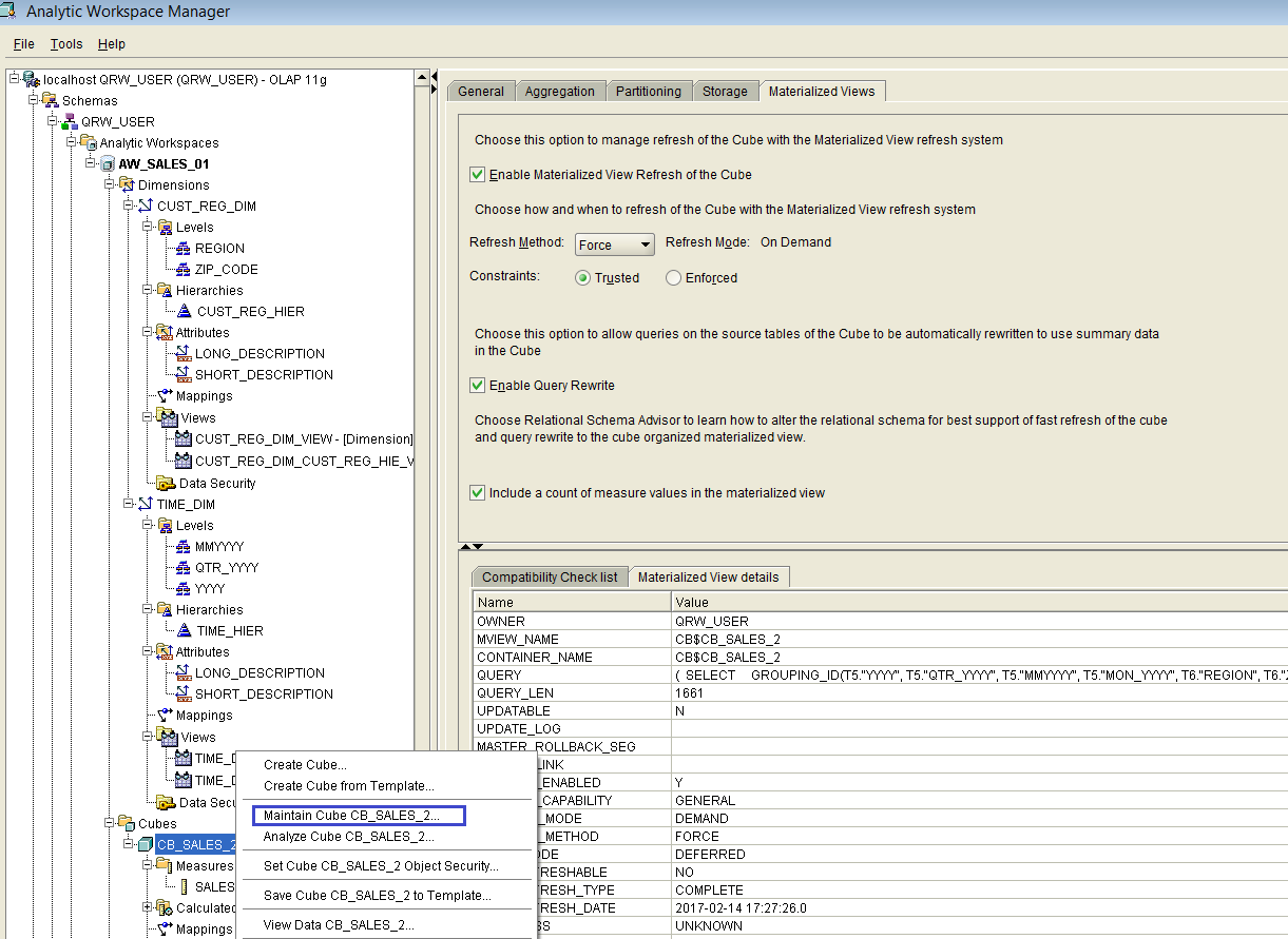
Figure 24 below shows the pop-up menu we get when we select the cube CB_SALES_2 and then we click the right button on the mouse.
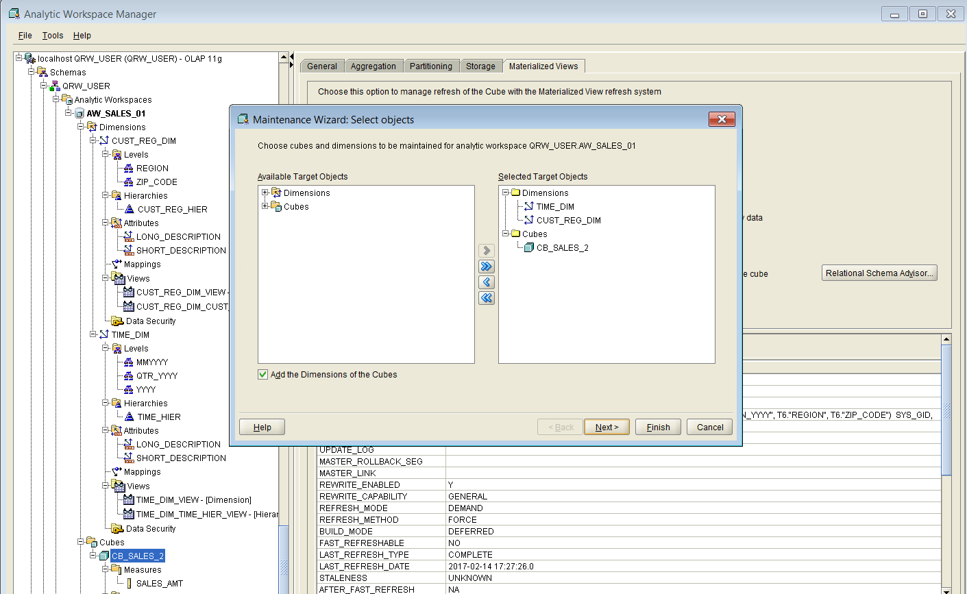
If we choose the item “Maintain Cube CB_SALES_2” from the pop-up menu, then a wizard-style window appears, as shown below in Figure 25.
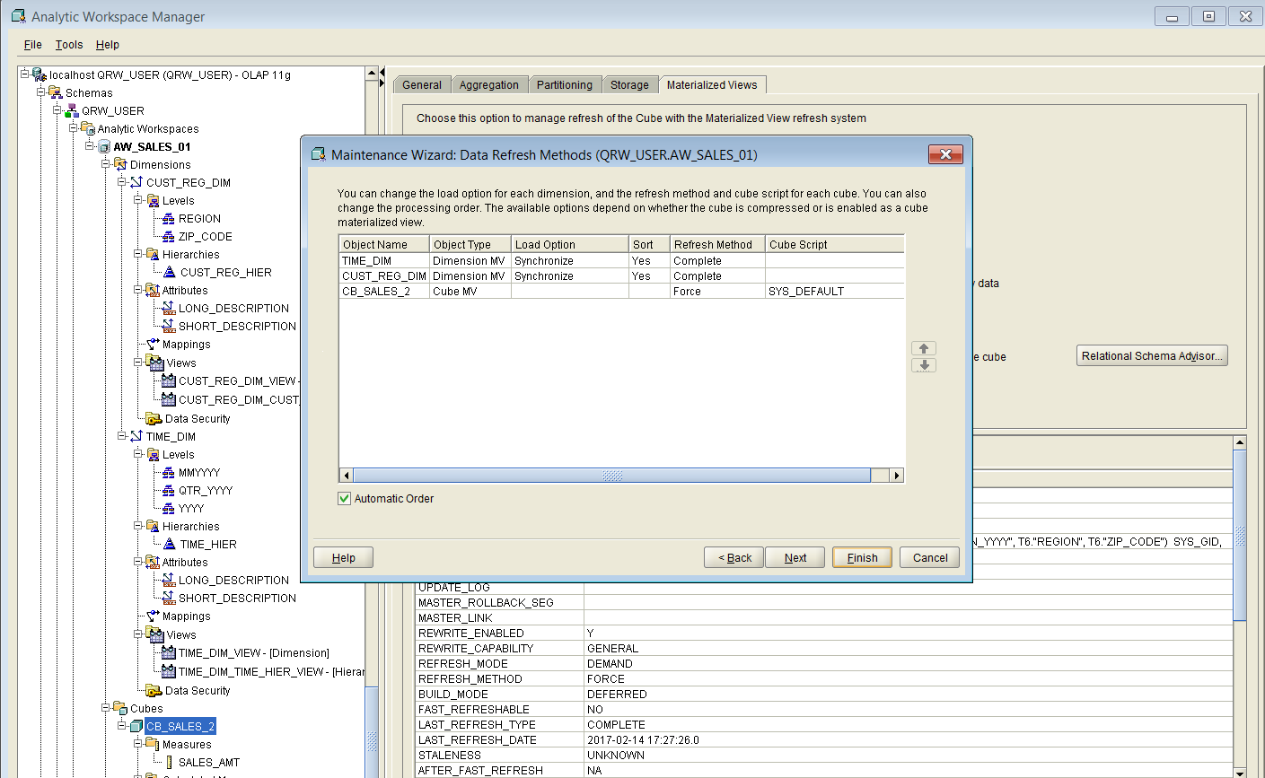
We select the dimensions and the cube in the left pane, and we add them to the right pane, as shown in Figure 25 above. Then we click on the “Next” button, which brings us to the second step of the wizard, as shown in Figure 26 below:
We can now click on the “Finish” button, which will initiate the loading of the selected dimensions and the cube, with data. If no errors have occurred, the cube should be loaded with aggregated data, and it should be available for query rewrite by the oracle optimizer.
Now, let’s verify that SQL query rewrite to the cube actually happens.
First of all, we need to check if there are any MV’s in schema QRW_USER and, if so, we need to disable query rewrite to those MV’s, in order to direct the optimizer to rewrite towards the cube.
The query below (let’s call it Q_SHOWMV) should list all the MV’s in the user’s schema, excluding the cube-organized MV’s:
select * from user_mviews

where mview_name not like 'CB%'

order by mview_name;
If the query (Q_SHOWMV) returns any rows (see example in Figure 27 above), we need to disable those MV’s for query rewrite, as shown in the example code below:
ALTER MATERIALIZED VIEW SALES_MV_TK

DISABLE QUERY REWRITE;
Now, we need to check that query rewrite is enabled for our session, as shown below:
select name, value from v$parameter

where name like 'query_rewrite_%'

order by name asc;
We need the parameter values to look like below:
If the values returned are different from what is shown in Figure 28, then please look at this page in order to see how to set them properly.
Now, let’s consider two SQL aggregation queries, (Q1) and (Q2), against a simple star schema, as shown below:
--(Q1)

SELECT

SUM(SALES_AMOUNT), TIME_HIERARCHY_TK.QTR_YYYY

FROM SALES_TK, TIME_HIERARCHY_TK

WHERE SALES_TK.TRANS_DATE = TIME_HIERARCHY_TK.DAY

GROUP BY TIME_HIERARCHY_TK.QTR_YYYY;
As we can see from the explain plan capture shown in Figure 29 below, this SQL query gets rewritten by the oracle optimizer to make use of the cube data, via the cube-organized materialized view called CB$CB_SALES_2:
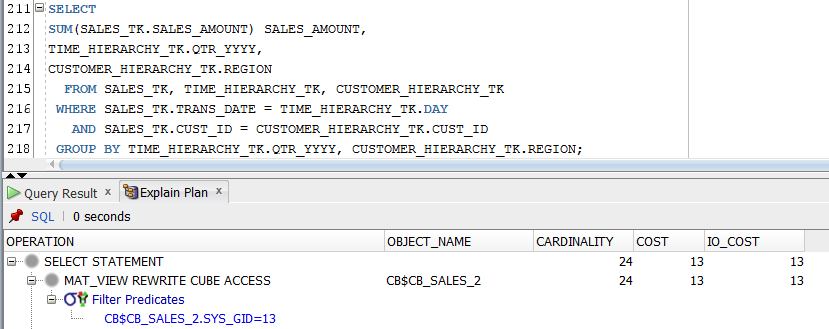
The SQL query (Q1) shown above uses one dimension (a subset of all dimensions available) to aggregate data. Below we can see another SQL query called (Q2), which aggregates data along two dimensions (all of the available dimensions in our case study of a simple star schema):
--Q2

SELECT

SUM(SALES_TK.SALES_AMOUNT) SALES_AMOUNT,

TIME_HIERARCHY_TK.QTR_YYYY,

CUSTOMER_HIERARCHY_TK.REGION

FROM SALES_TK, TIME_HIERARCHY_TK, CUSTOMER_HIERARCHY_TK

WHERE SALES_TK.TRANS_DATE = TIME_HIERARCHY_TK.DAY

AND SALES_TK.CUST_ID = CUSTOMER_HIERARCHY_TK.CUST_ID

GROUP BY TIME_HIERARCHY_TK.QTR_YYYY, CUSTOMER_HIERARCHY_TK.REGION;
As we can see from the explain plan capture shown in Figure 30 below, this SQL query also gets rewritten by the oracle optimizer to make use of the cube data, via the cube-organized materialized view called CB$CB_SALES_2:
To summarize: in our case study of a simple star schema with one fact table and two dimension tables, we have achieved SQL query rewrite to an OLAP cube via cube-organized MV’s, when we used all available dimensions, and also when we used a subset of all available dimensions.
In a future article I will explore in more detail the mechanisms used by the oracle database engine to store and access the data inside the cube.
The Blog is under construction, so please be patient and check daily for new content.
Stay tuned for more…
<< Prev Page | Next Page >>

